
This is a note on my Year 3 lab experiment analysing Z-boson dilepton production with ATLAS Open Data, written here in case I forget the details a few years from now.
I carried out this computational analysis with Hansheng Ye. The main work measured $Z\to e^+e^-$ and $Z\to\mu^+\mu^-$ production using 13 TeV ATLAS Open Data. My extension work started with an awkward dependence on the muon isolation cuts and ended with a deliberately simplified but practical FSR-inspired mass recovery.
The basic background
The reason $Z\to\ell^+\ell^-$ is such a useful collider process is that it leaves a clean signature inside otherwise messy proton–proton collisions. If two reconstructed electrons or muons came from a Z boson, their invariant mass should cluster around $m_Z\simeq91.19\ \mathrm{GeV}$:
$$m_{\ell\ell}^2=(p_{\ell^+}+p_{\ell^-})^2.$$
The invariant mass does not care how fast the Z was moving in the lab frame. Get the two lepton four-vectors right and the peak appears.
The collision data tell us how many events were actually recorded. Monte Carlo samples do the jobs that data cannot do by themselves: they estimate selection efficiency, model the expected shapes, and account for backgrounds. The signal samples here were $Z\to ee$ and $Z\to\mu\mu$; the main backgrounds included low-mass Drell–Yan, $Z\to\tau\tau$, $t\bar t$, and W+jets. Every MC event carried a weight, so simply counting rows was not enough.
Isolation is the other piece of background worth recalling. A prompt lepton is usually not surrounded by much extra activity, whereas a lepton produced inside a jet often is. We used two cone variables:
lep_ptvarcone30, the transverse-momentum sum of nearby tracks;lep_topoetcone20, the transverse-energy sum of nearby calorimeter clusters.
Tighter isolation rejects more background, but it can also reject real signal. Final-state radiation makes this especially annoying: a lepton can radiate a nearby photon after the Z decay, and that photon can contribute to the calorimeter isolation even though the event is still a genuine $Z\to\ell\ell$ event.
What the main analysis actually did
I first applied a baseline preselection to the full samples and wrote the variables needed later into reduced parquet files. That made the cut scans manageable; I did not have to reprocess the original ntuples every time I moved a threshold.
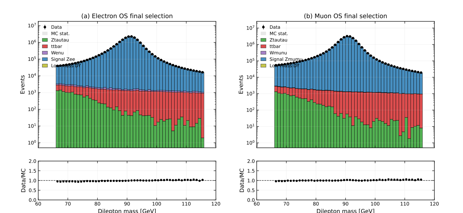
The analysis was deliberately split into two stages. During the build stage, the code kept events with exactly two leptons of the required flavour, applied the baseline $p_T$, trigger, and identification requirements, constructed the dilepton four-vector, and stored mass and the lepton charge product alongside the isolation variables. During the analysis stage, the reduced parquet files could be read repeatedly for the opposite-sign and same-sign selections, isolation scans, mass-window variations, and control-region checks. The MC event-weight field was retained when the samples were slimmed, which mattered for every yield and efficiency calculated later.
The final event selection was roughly:
- exactly two reconstructed leptons;
- same flavour and opposite charge;
- the appropriate lepton trigger had fired;
- baseline $p_T$ and Medium identification requirements;
- $66<m_{\ell\ell}<116\ \mathrm{GeV}$;
- track and calorimeter isolation for both leptons.
The final isolation working points were:
| channel | ptvarcone30 maximum |
topoetcone20 maximum |
|---|---|---|
| electron | 4.5 GeV | 9.25 GeV |
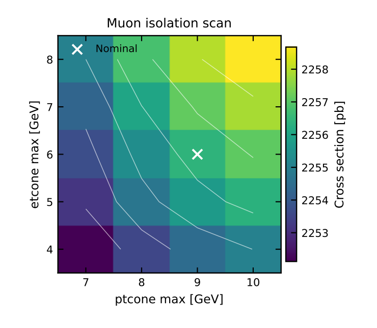
| muon | 9.0 GeV | 6.0 GeV |
The cross section was extracted from
$$\sigma=\frac{N_{\mathrm{selected}}-N_{\mathrm{background}}}{\epsilon\int\mathcal{L}(t)\mathrm{d}t}.$$
where the efficiency $\epsilon$ came from signal MC and the integrated luminosity was $30.6\ \mathrm{fb}^{-1}$.
More explicitly, the numerator used the unweighted number of selected data events minus the weighted MC background yield. The efficiency was the weighted signal yield passing the full selection divided by the total produced signal sum of weights. This is easy to forget when looking only at the final formula: the data count, background estimate, and efficiency do not all come from the same kind of counting.
The results were:
| channel | measured cross section |
|---|---|
| $e^+e^-$ | $2203.1\pm0.5\ (\mathrm{stat.})\pm9.3\ (\mathrm{syst.})\pm37.5\ (\mathrm{lumi.})\ \mathrm{pb}$ |
| $\mu^+\mu^-$ | $2248.3\pm0.5\ (\mathrm{stat.})\pm13.7\ (\mathrm{syst.})\pm38.2\ (\mathrm{lumi.})\ \mathrm{pb}$ |
The samples were large enough that the statistical uncertainty was tiny. The dominant uncertainty was the 1.7% luminosity uncertainty. The quoted systematic uncertainty was a selection-dependence estimate: I varied the mass window and isolation cuts, then kept the largest shift in the extracted cross section. Isolation dominated that estimate in both channels.
The electron and muon results differ by about 2%. They probe the same underlying process, but the detector response, reconstruction, identification, and isolation behaviour are not the same, so I kept the channels separate rather than forcing a combined number.
I also looked at wrong-flavour and wrong-charge regions as checks for unmodelled background. The electron result could move by as much as roughly 24 pb, but the same-sign electron region is contaminated by charge misidentification and signal leakage. It was useful as a warning, not clean enough to become the quoted background systematic.
Why I ended up looking at FSR
The extension began with a scan of the muon isolation thresholds. Loosening ptvarcone30 and topoetcone20 made the extracted cross section rise. In other words, the extra events entering the selection were not behaving exactly as the signal efficiency and background prediction said they should.
I made a control sample of opposite-sign dimuon events that failed the nominal $(9,6)\ \mathrm{GeV}$ isolation but passed a looser $(15,15)\ \mathrm{GeV}$ requirement. Its raw $m_{\mu\mu}$ distribution showed a clear data excess on the low-mass side of the Z peak.
In the dedicated FSR run, this control sample contained 568,770 data events. The corresponding weighted MC prediction was about 381,210 signal events plus 7,773 background events, leaving an overall data–MC excess of roughly 179,787 events. The size of that mismatch made it unlikely that I was only looking at a small statistical fluctuation.
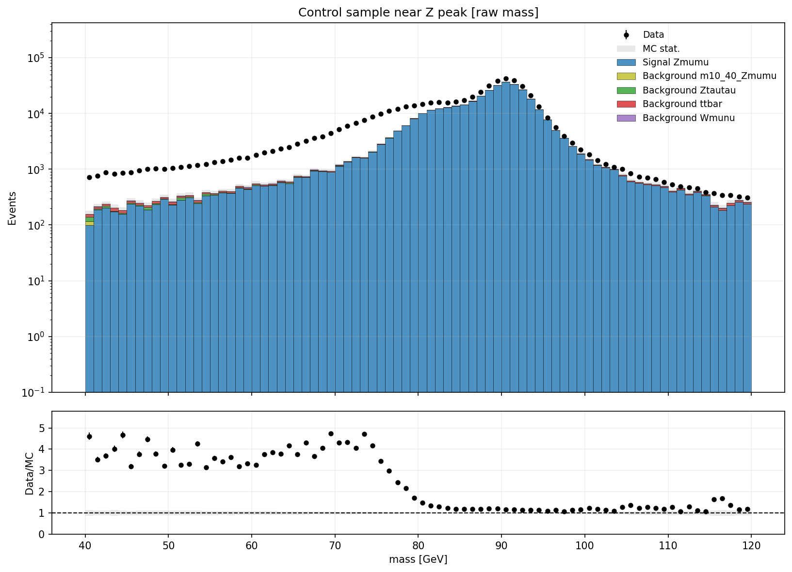
FSR gives a plausible way to connect the two observations. If a muon radiates a photon and the photon energy is not included in the muon four-vector, the reconstructed dimuon mass moves below the Z peak. If that photon sits near the muon, it can also increase topoetcone20 and make the event fail isolation.
The toy recovery
This was not the ATLAS FSR reconstruction. I had no reconstructed photon candidate, no photon identification, and no proper angular matching. The test was much narrower: if some of the energy in the isolation cone came from FSR, would adding it back move the excess in the expected direction?
For control-sample events with raw $m_{\mu\mu}<80\ \mathrm{GeV}$, I took the muon with the larger lep_topoetcone20. I treated that scalar cone energy as a proxy for nearby radiation, assumed it was collinear with the muon, added it to the muon four-vector, and recalculated the mass. In the code, the proxy energy $\Delta p_T$ changed the selected muon according to
$$p_T’ = p_T + \Delta p_T, \qquad E’ = E + \Delta p_T\cosh\eta,$$
while keeping its $\eta$ and $\phi$ fixed. The dimuon mass was then rebuilt from the corrected pair. Data and MC received exactly the same treatment.
The FSR study used a dedicated parquet containing the full lepton four-vector fields needed for this recalculation. It was processed sample by sample and parquet row group by row group; the plotting code accumulated histogram bins instead of materialising every selected event from every sample in memory. That implementation detail is not part of the physics result, but it explains how the full-fraction study remained practical on a laptop.
The excess moved rather than vanished:
| mass region | data−MC excess before | data−MC excess after |
|---|---|---|
| 66–80 GeV | $7.2\times10^4$ | $1.6\times10^4$ |
| 80–100 GeV | $6.2\times10^4$ | $1.3\times10^5$ |
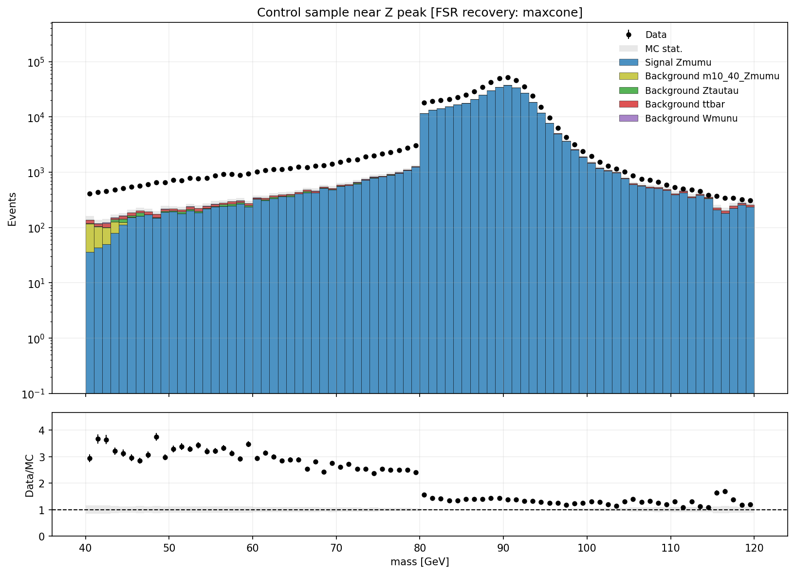
The low-mass excess was strongly reduced and the higher-mass region gained events. That is consistent with missing near-muon energy being moved back towards the Z peak. It supports an FSR-like interpretation of the isolation-fail sample, but it does not establish that every recovered event contained an FSR photon.
More importantly, this mass-only recovery did not remove the dependence of the final cross section on the isolation working point. I therefore kept it as a diagnostic and did not use the corrected mass in the headline measurement.
The code also contained two useful cross-checks that did not make it into the headline result. One added the cone proxy to both muons rather than only the larger-cone muon. Another used the maxcone mass correction and subtracted the same proxy from the calorimeter-isolation value before reapplying the selection. The second version was a more direct toy test of an FSR-aware isolation definition, but it also shifted the selected yield and the extracted normalisation. In the dedicated FSR workflow, the raw and mass-only nominal values were almost identical, while the etcone-subtracted variant moved the result by about 14 pb. That was another reason not to present it as a calibrated correction.
Why it was only a diagnostic
topoetcone20 is a scalar cone sum, not a photon four-vector. It can contain pile-up, underlying-event activity, and calorimeter noise as well as radiation. Treating the whole sum as one collinear photon is physically crude.
The $m_{\mu\mu}<80\ \mathrm{GeV}$ condition also sculpts the corrected distribution. I chose 80 GeV to isolate the shoulder I was investigating; it is not a natural boundary in the physics.
There is a deeper consistency problem too. The recovery shown in Figure 4 changed the reconstructed mass but not the isolation definition. If photon energy is what made the event fail isolation, a proper recovery should identify that photon before selection and remove its contribution from the isolation variable where appropriate. The etcone-subtracted cross-check tried this idea in the crudest possible way, but a cone sum is still not a reconstructed photon. Neither version was sufficient to stabilise the cross section.
Finally, I did not use truth information to check whether the recovered energy actually came from FSR. That is why I called the exercise FSR-inspired rather than an FSR measurement.
What I would do next
If I returned to this analysis, I would start from signal MC truth and measure how often genuine FSR photons appear in the low-mass isolation-fail sample. I would then use reconstructed photons or individual calorimeter clusters, match them to muons with $\Delta R$, and perform the recovery before applying isolation. The mass and isolation variables would be recalculated together.
I would also compare unrecovered, FSR-tagged, and recovered events at truth and reconstruction level, check the mass closure, and vary or remove the hard 80 GeV boundary. Only after that would I ask whether the recovery makes the extracted cross section more stable under isolation changes.
The useful part of this extension was not that I “fixed FSR”. I noticed a dependence in a cut scan, isolated the events responsible for it, and tested a physical explanation against the shape of the data. The test was crude, but the low-mass excess responded exactly where an FSR-like effect should respond. That is the part I do not want to forget.